13.1 Introduction to Partial Differential Equations
We have previously discussed a lot of linear algebra and complex analysis, and we have seen how these topics are useful in physics. In this section, we will introduce the topic of partial differential equations (PDEs), which are equations that involve functions of multiple variables and their partial derivatives. PDEs are ubiquitous in physics; almost every field of physics uses PDEs to describe physical phenomena. In electrostatics, we have Poisson's equation (in Gaussian units)
and in electrodynamics, we have Maxwell's equations
The wave equation
is used to describe wave propagation, and the Schrödinger wave equation
is used to describe quantum mechanical systems.
Table of Contents
Separation of Variables
The first step in solving a PDE is to find a way to reduce the problem to a simpler one. One common technique is to use the method of separation of variables, which involves assuming that the solution can be written as a product of functions, each depending on only one of the variables. We typically assume that the solution can be written as
where
The temporal component is usually a first or second order derivative, so most of our PDEs will look like
So we have, after separating variables,
We can then divide both sides by
As the left-hand side depends only on the spatial coordinates and the right-hand side depends only on time, the only way this can be true is if both sides are equal to a constant, which we will denote by
Notice that the time-dependent part of the equation is a first or second order ODE. The spatial part reduces to a PDE of the form
Generally, our expression for
where
And rewriting
We have a homogeneous PDE, which we typically solve using further separation of variables. The rest of these sections will be devoted to separation of variables in different coordinate systems.
Separation of Angular Variables
Define the momentum operator
The angular momentum operator is defined as
The commutation relations for the angular momentum operator are given by
The reason we are interested in the angular momentum operator is that it is dependent only on the agular variables
To proceed, we need to symmetrize the terms (so that we can collapse them back into a dot product). Therefore we use the commutation relations to write
which simplifies to
Finally, substituting back
Rearranging this expression, and noting that
So we have two important results here; first is a coordinate-independent expression for the Laplacian operator in terms of the angular momentum operator, and second is the expression for the Laplacian operator in spherical coordinates:
Going back to our homogeneous PDE
Let's now perform further separation of variables by assuming that
Assuming, once again, that
(See the appendix for a justification of this step.)
Letting the first term be
The second equation is an ODE for the radial part
Eigenvalues of L² in Abstract Space (Ladder Operators)
Let's consider an abstract vector space where a ket
Since
Recall that a degenerate eigenvalue is one that corresponds to multiple linearly independent eigenvectors. In order to distinguish between these eigenvectors, we need to find another operator that commutes with
Anyways we have
where
In order to find the possible values of
and they are Hermitian conjugates of each other, i.e.,
Since
To verify that ladder operators do indeed raise and lower the eigenvalues of
and similarly,
Combining these results, we see that
with
Restricting the Eigenvalues
To find the possible values of
First, we note that
so
Next, we can express
and similarly,
Adding these two expressions together gives
Therefore we have
which simplifies to
Since
As the norm term is non-negative, we have
We can add these two inequalities together to get
So this places a restriction on the possible values of
Plugging in
and plugging in
Solving these two equations simultaneously gives
We must have
The takeaway is this: if we have any eigenvector
This means that
Since
Substituting this back into the expression for
These results can be stated in theorem form.
The eigenvalues of the operator
where
We also need to address the normalization of the eigenvectors. We know that the eigenvalues of
Let's find the norm of the laddered eigenvectors. We have
Thus,
Substituting in the earlier expression for
We drop the phase factor by choosing
The action of the ladder operators on the eigenvectors
Let
We can find a closed-form expression for the eigenvectors
Eigenvalues of L² in Function Space (Spherical Harmonics)
Now we can return to the original problem of finding the angular part of the solution
Let's consider each component of the angular momentum operator in spherical coordinates. The eigenvalue equation for
Let's separate variables by assuming that
This is an ODE for
where
Integer Values of m
We will first consider the case where
We will need to find expressions for the ladder operators in spherical coordinates. Using the earlier expressions for
Recall that
This simplifies to
which is an ODE for
So the highest eigenfunction is
To find the rest of the eigenfunctions, we simply apply the lowering operator
It can be shown that applying the term in parentheses gives
So using that and
Repeatedly applying the lowering operator will lead to the general expression
where we have made the substitution
Finally, we can determine the normalization constant
This is just the Legendre polynomial
so we can use the normalization condition for Legendre polynomials to find
(the completeness relation for spherical coordinates), we have
Substituting
It can be shown that this leads to
Thus, the final expression for the eigenfunctions is
with
The
but for historical reasons, we use the associated Legendre functions defined by
We thus have
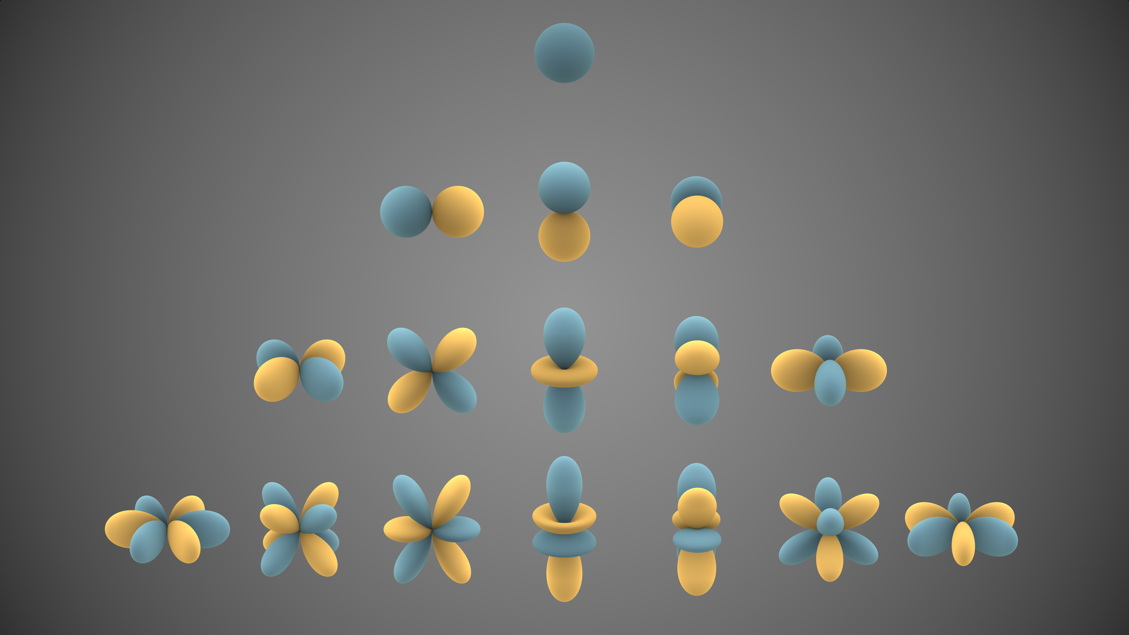
The spherical harmonics, which are solutions to the angular part of the Laplace equation in spherical coordinates, are given by
where
Appendix: L Only Depends on Angular Variables
To justify the step where we assumed that
Let
Let's convert this to spherical coordinates using the respective transformations
Using the chain rule, we have
Calculating the partial derivatives (using the transformations above), we have
Now we can use these expressions to rewrite
so
Similarly, for
so
Finally, for
so
Now we can compute
Similarly, for
And for
Adding these three expressions together, we have
In the last step we used a reverse product rule to rewrite the first two terms.
This final expression for